Packed-bed model

PackedBedModel describes a bed of spherical PCM capsules with the heat transfer fluid flowing through the voids. At each point along the bed, heat conducts across a capsule (resolved radially) and into the fluid at its surface. It is built from the same submodels as the finned-tube models, so it has the same outputs, conserves energy exactly and runs the same experiments.

The default parameters are the experiments of Nallusamy et al. (2007): a 47 l tank of paraffin capsules in water, charged with water at 70 °C from 32 °C.

For the geometry, the equations and the options of the packed-bed model, with sketches, see the Packed bed page of the documentation.

Tutorial 3 introduces this model.

import matplotlib.pyplot as plt
import numpy as np
import pybamm

import pytes

model = pytes.PackedBedModel()
model.print_submodel_info()

fluid: AdvectedFluid (Heat transfer fluid)
    requires:
        Heat transfer fluid heat gain per unit length [W.m-1]
        Initial uniform temperature [K]
    provides:
        Heat transfer fluid specific enthalpy [J.kg-1]
        Inlet specific enthalpy [J.kg-1]
        Outlet specific enthalpy [J.kg-1]
        Mass flow rate [kg.s-1]
        Heat transfer fluid thermal energy [J]
        Heat transfer fluid temperature [K]
        Inlet temperature [K]
        Outlet temperature [K]
        Inlet-outlet temperature difference [K]
        Heat transfer fluid velocity [m.s-1]
        Volume flow rate [m3.s-1]
        Pumped volume [m3]
    parameters:
        Bed cross-sectional area [m2]
        Bed length [m]
        Bed porosity
        Heat transfer fluid density [kg.m-3]
        Heat transfer fluid specific heat capacity [J.kg-1.K-1]
        Inlet temperature [K]
        Mass flow rate [kg.s-1]
        PCM melting temperature [K]
        Reference temperature [K]
    assumptions:
        The fluid is incompressible, with constant density.
        Axial conduction and dispersion in the fluid are neglected.
        The flow is the same in every flow path.
storage: EnthalpyStorage (Phase-change material storage)
    requires:
        Phase-change material boundary heat flux [W.m-2]
        Initial uniform temperature [K]
    provides:
        Phase-change material enthalpy [J.m-3]
        Phase-change material enthalpy rate of change [W.m-3]
        Phase-change material conduction heating rate [W.m-3]
        Phase-change material thermal energy [J]
        Liquid fraction
        Phase
        Average liquid fraction
        Phase-change material temperature [K]
        Phase-change material average temperature [K]
        Phase-change material cross-section average temperature [K]
        Phase-change material surface temperature [K]
        Phase-change material thermal conductivity [W.m-1.K-1]
    parameters:
        Bed cross-sectional area [m2]
        Bed porosity
        Capsule radius [m]
        PCM latent heat [J.kg-1]
        PCM liquid phase conductivity [W.m-1.K-1]
        PCM liquid phase density [kg.m-3]
        PCM liquid phase specific heat capacity [J.kg-1.K-1]
        PCM melting range [K]
        PCM melting temperature [K]
        PCM smoothing width [K]
        PCM solid phase conductivity [W.m-1.K-1]
        PCM solid phase density [kg.m-3]
        PCM solid phase specific heat capacity [J.kg-1.K-1]
        Reference temperature [K]
    assumptions:
        Heat flows along the primary spatial variable only.
        Heat flows by conduction only (no convection in the liquid).
        The volume change on melting is neglected.
coupling: WallCoupling (Wall coupling)
    requires:
        Phase-change material conduction heating rate [W.m-3]
        Heat transfer fluid specific enthalpy [J.kg-1]
        Heat transfer fluid temperature [K]
        Phase-change material surface temperature [K]
        Mass flow rate [kg.s-1]
    provides:
        Heat transfer fluid heat gain per unit length [W.m-1]
        Phase-change material boundary heat flux [W.m-2]
        Heat transfer coefficient [W.m-2.K-1]
        Surface Reynolds number
        Surface Prandtl number
    parameters:
        Bed cross-sectional area [m2]
        Bed porosity
        Capsule radius [m]
        Heat transfer coefficient [W.m-2.K-1]
        Heat transfer fluid conductivity [W.m-1.K-1]
        Heat transfer fluid specific heat capacity [J.kg-1.K-1]
        Heat transfer fluid viscosity [Pa.s]
    assumptions:
        (none)
device energy: DeviceEnergy (Device energy)
    requires:
        Mass flow rate [kg.s-1]
        Outlet specific enthalpy [J.kg-1]
        Inlet specific enthalpy [J.kg-1]
        Phase-change material thermal energy [J]
        Heat transfer fluid thermal energy [J]
        Phase-change material average temperature [K]
        Phase-change material cross-section average temperature [K]
    provides:
        Power [W]
        Discharged energy [J]
        Charged energy [J]
        Discharged throughput [J]
        Charged throughput [J]
        Storage thermal energy [J]
        Total thermal energy [J]
        Heat loss power [W]
        Storage average temperature [K]
        Storage cross-section average temperature [K]
        Initial uniform temperature [K]
    parameters:
        Initial temperature [K]
    assumptions:
        There are no heat losses to the surroundings.
per-area totals: PerAreaTotals (Per-area totals)
    requires:
        Power [W]
        Discharged energy [J]
        Storage thermal energy [J]
        Total thermal energy [J]
    provides:
        Power per unit area [W.m-2]
        Discharged energy per unit area [J.m-2]
        Storage thermal energy per unit area [J.m-2]
        Total thermal energy per unit area [J.m-2]
    parameters:
        Bed cross-sectional area [m2]
    assumptions:
        (none)
geometry parameters:
    Bed length [m]
    Capsule radius [m]

t_end = 160 * 60
solution = pybamm.Simulation(model).solve(
    [0, t_end], t_interp=np.linspace(0, t_end, 321)
)
E = solution["Total thermal energy [J]"].entries
discharged = solution["Discharged energy [J]"].entries
print("max conservation error [J]:", np.max(np.abs(E - E[0] + discharged)))
print("stored energy [kWh]:", E[-1] / 3.6e6)
print(
    "energy between 32 and 70 degC [kWh]:",
    pytes.energy_between(model, 273.15 + 32, 273.15 + 70) / 3.6e6,
)
print(
    "stored energy per unit area [MJ.m-2]:",
    solution["Total thermal energy per unit area [J.m-2]"].entries[-1] / 1e6,
)

max conservation error [J]: 2.60770320892334e-08
stored energy [kWh]: 2.318240801224132
energy between 32 and 70 degC [kWh]: 2.635389843901675
stored energy per unit area [MJ.m-2]: 81.99099617603031

The measured fluid temperatures at a quarter, half, three quarters and the full height of the bed (points) against the model (lines).

Z = model.default_parameter_values["Bed length [m]"]
fig, ax = plt.subplots(figsize=(6, 4))
for position, fraction in [("0.25L", 0.25), ("0.5L", 0.5), ("0.75L", 0.75), ("1L", 1)]:
    t_data, T_data = np.loadtxt(
        f"data/Nallusamy2007_HTF_{position}.csv", delimiter=",", skiprows=1, unpack=True
    )
    t = solution["Time [s]"].entries
    T = solution["Heat transfer fluid temperature [degC]"](t=t, z=fraction * Z)
    (line,) = ax.plot(t / 60, T, label=f"{fraction:g} L")
    ax.plot(t_data, T_data, "o", color=line.get_color(), markersize=3)
ax.set_xlabel("Time [min]")
ax.set_ylabel("Fluid temperature [°C]")
ax.legend()
plt.show()

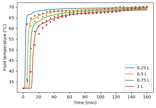
The fluid temperatures agree with the measurements to within 2 K (root mean square: 0.98, 0.68, 1.41 and 1.85 K at a quarter, half, three quarters and the full height). Inside the capsules the agreement is looser, about 5 K at 0.8 of the capsule radius, which depends on where the thermocouples sat and on the capsule shell, which the model neglects.

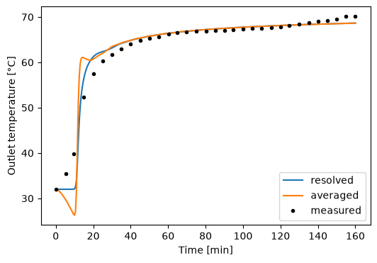
With options={"storage along flow path": "averaged"}, one capsule stands for the average along the bed and exchanges heat with the fluid averaged along it: much faster, but it cannot capture the thermal front moving through the bed. Every model has this option.

Note the dip of the averaged outlet below the initial 32 °C early on, and the smaller one (about 0.6 K) just after it peaks. Both come from the heat the capsule takes from the averaged fluid, which is taken uniformly along the bed. Early on, that includes the outlet, where the fluid is still cold. Later, as hot fluid fills the bed, the averaged fluid warms, and the capsule takes more heat everywhere, cooling the fluid it had already warmed. Neither dip changes with the mesh: they are known artefacts of this formulation, the published reduced model; energy is still conserved exactly.

averaged = pytes.PackedBedModel(options={"storage along flow path": "averaged"})
averaged_solution = pybamm.Simulation(averaged).solve(
    [0, t_end], t_interp=np.linspace(0, t_end, 321)
)
print(
    f"solve time: resolved {solution.solve_time}, averaged {averaged_solution.solve_time}"
)

t_data, T_data = np.loadtxt(
    "data/Nallusamy2007_HTF_1L.csv", delimiter=",", skiprows=1, unpack=True
)
fig, ax = plt.subplots(figsize=(6, 4))
for sol, label in [(solution, "resolved"), (averaged_solution, "averaged")]:
    ax.plot(
        sol["Time [min]"].entries, sol["Outlet temperature [degC]"].entries, label=label
    )
ax.plot(t_data, T_data, "ko", markersize=3, label="measured")
ax.set_xlabel("Time [min]")
ax.set_ylabel("Outlet temperature [°C]")
ax.legend()
plt.show()

solve time: resolved 1.653 s, averaged 77.659 ms